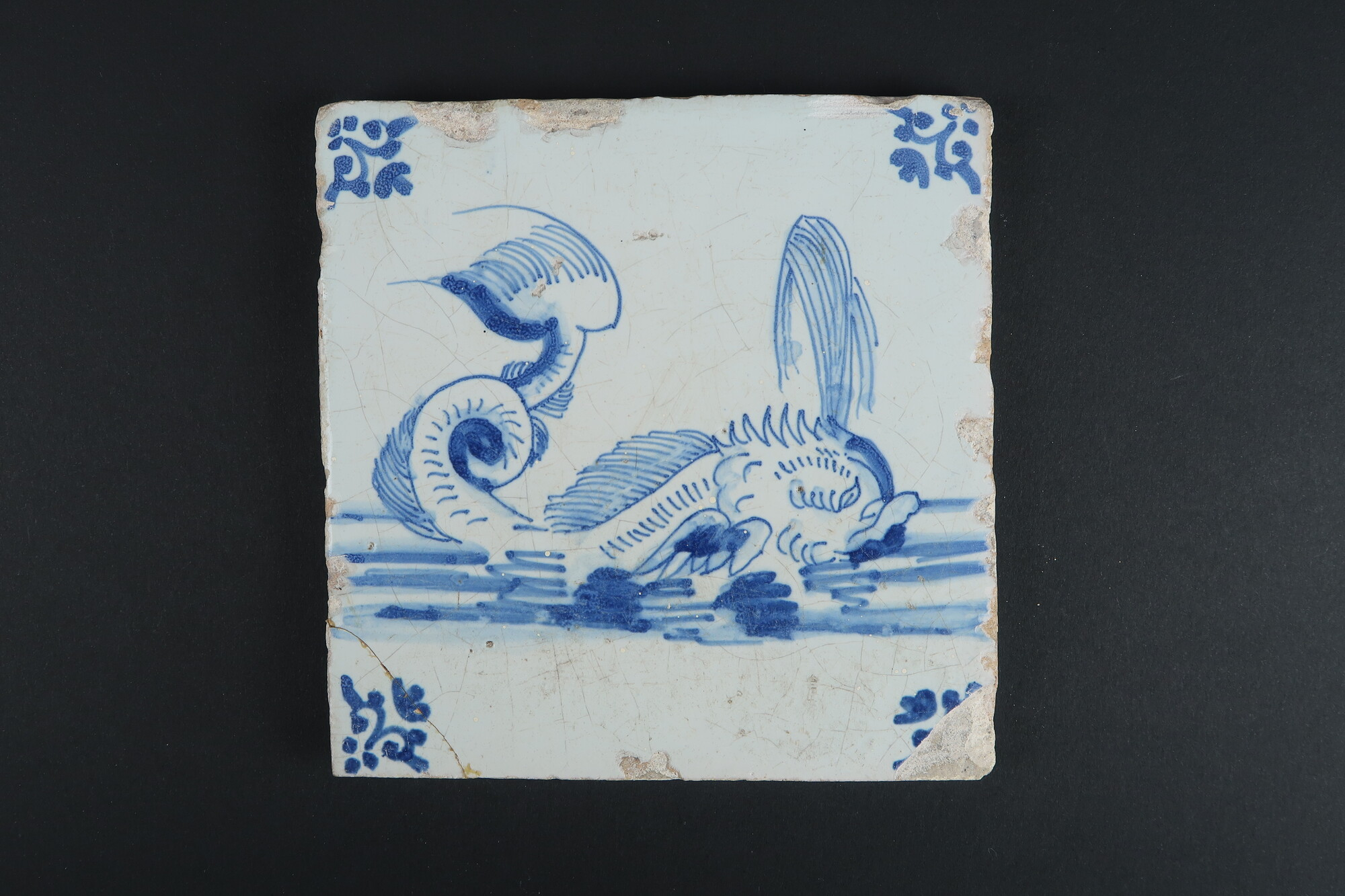
The museum was founded in 1903 to be open to anyone who
wanted to draw, study, copy and remake what it held. This API is that
invitation in a digital form.
This URI content-negotiates: request it with
Accept: application/ld+json to be redirected to the catalog.
An index is not the collection. It is a way in — a list of handles
that lets you reach for one thing among many without looking at
everything first. Every index is a decision about what is worth finding,
and that decision is made long before anyone searches.
Museums have always indexed. The card catalogue, the register, the
thesaurus: each one fixes a small set of properties — maker, material,
date, type — and makes those properties findable at the cost of
everything it leaves out. What a period chose to record tells you what
that period thought a collection was for. The gaps are as legible as the
entries.
Those indexes were made by hand, so they had to be economical. A
cataloguer could not record the colour of ten thousand objects, or how
much of each object that colour covered, and no one asked them to. The
limit was labour, and the categories grew around it.
Machines lift that limit, and in doing so they make new kinds of
index possible: properties nobody catalogued because cataloguing them
was never practical. This is not a better index, and it does not replace
the ones made by hand. It measures something different, with its own
blind spots — a colour index describes photographs as much as it
describes objects, and it knows nothing of what any of these things
mean. What it offers is another way in, and a set of questions the
existing categories were not shaped to ask.
What follows are indexes of that second kind, built from the
collection data and open for anyone to query, reuse or disagree
with.
One caveat throughout. These indexes describe the objects
published through this API — around ten thousand of the twenty-four
thousand the museum holds. Which objects have been published, and in what
order, is itself a decision made by people, and it shapes every figure
below. This is a view of the catalogue, not of the collection.
Colour
Colours are extracted from the digital images: the
background
is removed, the remaining pixels are clustered, and each cluster is
matched to a named tone and a broad base colour. What you see below is how
much of the collection's visible surface each colour accounts for.
The collection's palette
Twelve broad categories. Every colour the
tagger finds is assigned to one of twelve base names — red, orange,
brown, grey and so on — and the band shows how much of the collection's
visible surface each accounts for. It is deliberately coarse: it answers
"how much of this collection is blue" without pretending the answer is
precise. Click a segment to see the tones it is made of, and the objects
it dominates.
The same measurements, ungrouped. Each
colour cluster is matched to the nearest name from an extended colour
list — several hundred of them, from Davy's grey to Fuzzy Wuzzy — and
kept separate rather than folded into a base. This is the finer
reading: it distinguishes tones the twelve categories flatten together,
at the cost of a long tail where most names sit on only a handful of
objects. The twelve categories are these tones, grouped.
Objects
Time
Two different times run through a collection. There is
when each object was made, and there is when the museum took it in. They are
rarely the same, and the distance between them is collecting policy made
visible.
Two readings of time
Above the line: when the objects were made.
Nearly every published object carries a production date, but only a
quarter carry an exact year — the rest are spans, some a century wide.
Rather than pinning those to their first year, each object spreads a
single unit of weight evenly across the years it might have been made
in. An object dated 1937 puts its whole weight on one year; one dated
1900/2000 puts a hundredth on each of a hundred. So height is share,
not certainty, and vague dating shows as flatness rather than as a
false spike. The darker band is the objects dated to a single year,
which says as much about when record-keeping became precise as about
the objects themselves.
Below the line: when they entered the
collection. An acquisition date is a point, not a span — the
museum took the object on one day — so this is a plain count with no
weighting. It is deliberately spiky: collections grow in events, and a
single bequest or purchase can bring in hundreds of objects on one
date. Note that the line begins only in 1904, a year after the museum
was founded, and that around a quarter of published objects carry no
acquisition date at all.
Reading the gap. Where the upper shape
runs ahead of the lower one, the museum was collecting objects made
long before — the 1980s took in more objects than any other decade,
most of them decades old already. After 2010 the relationship
inverts. And both shapes thin sharply through the 1930s and 1940s:
the collection neither acquired much then nor holds much made then.
Made — all dated objects, weighted by span
Made — dated to an exact year
Acquired — objects entering the collection
Each bar is a decade of acquiring. It is
divided by how old the objects were when the museum took them in, and
its height is the number of objects — so the decades that collected
little are visibly slight, rather than given the same authority as the
ones that collected thousands.
The age is a range, not a number. An
object recorded as made between 1900 and 1950 and acquired in 1907 was
somewhere between nought and seven years old — the 1950 was an
open-ended note, and the purchase itself is evidence. Each object is
banded on the midpoint of its possible range, which is an estimate.
The purple rule under a bar is the share whose dating is too loose to
band confidently, and it is widest exactly where the collection is
largest.
It changes direction more than once. The
museum opened buying antiques, turned to the design of its own moment
within twenty years, swung back to the historical, and reached its
most contemporary in the 1990s — when half of everything acquired had
been made that same year. Since 2010 it has been turning again.
5 years old or less
6–25
26–100
Over a century
Too loosely dated to band
Resemblance
The other two indexes sort the collection into
categories. This one does not sort it at all. It measures how close any two
photographs sit in a space built by a machine that has looked at several
hundred million captioned images — and lets you walk from one object to its
nearest neighbours, and on from there.
Following a thread
There is no overview here, and that is the
point. Colour and time can be summarised in a single band, because
every object has a colour and a date. Resemblance is relational: it only
exists between things. So there is no picture of the whole — only a
starting object and what sits nearest to it, and then whatever sits
nearest to that.
What the machine is doing. Each photograph
is turned into a list of 768 numbers by CLIP, a model trained on images
paired with the text found near them online. Images described in similar
ways end up close together. Nothing here was catalogued: the model was
never shown this collection, never told what a decorative tile is, and
has no access to any record. It compares pictures.
What it therefore cannot know. It brings the
internet's associations with it, including its blind spots and its
clichés, and it will happily group objects for reasons that have nothing
to do with design history — a shared backdrop, a similar crop, a
photographic convention. It is not a judgement about the objects. It is
a measurement of their pictures, and it is worth disagreeing with.
Removing the background
A photograph is mostly not the object. Studio backdrops,
shadow and floor can take up more of the frame than the thing being
photographed, and a colour reading from the whole image describes the
photography as much as the collection. The background is removed before the
pixels are clustered.
1975-0061, as photographed. The frame the colour
tagger receives: the object, and everything around it.
Read from the whole frame. Each band is one colour
cluster, its width the share of pixels it covers. Backdrop and shadow
count as part of the object.Read from the object alone. The same clustering
after the background is masked out. This is what the index is built
from.